Manhattan College Business Analytics Competition 2023
1. Official poster: 2. Background story: 3. Data source: 4. Research links: https://education.nationalgeographic.org/resource/paradox-undernourishment Food Safety status in African countries https://agrilinks.org/post/advancing-food-safety-africa-opportunities-and-action-areas 5. The development of Food Safety in Sub-Saharan Africa: Based on the data found and researches, we concluded that Food Safety issue in Sub-Saharan Africa was determined by 2 main factors: Food Quantity and Food […]
1. Official poster:
2. Background story:
3. Data source:
4. Research links:
https://education.nationalgeographic.org/resource/paradox-undernourishment
https://agrilinks.org/post/advancing-food-safety-africa-opportunities-and-action-areas
5. The development of Food Safety in Sub-Saharan Africa:
Based on the data found and researches, we concluded that Food Safety issue in Sub-Saharan Africa was determined by 2 main factors: Food Quantity and Food Quality. As we developed deeper analysis on each factor, we found that there was no sufficient data to support Food Quality. Therefore, we decided to primarily focus on Food Quantity.
6. Indicator for Food Quantity & Other variables:
- We chose The Prevalence Number of Undernourished People in 20 years (2001 – 2020) as an indicator for Food Quantity (Y)
- We chose randomly a certain number of factors as variable X that we believed to have an impact on Food Quantity (Y)
7. Data cleaning:
We used R Studio to merge data tables from Excel files and convert rows to columns. Then we removed any variables that had more than 10% of missing values. That helped us to narrow down the number of variable X that was finally used for the analysis.
8. My major tasks: Gather data, Clean data, Develop K-means clustering analysis on the regional level.
- R script for Data Cleaning
library(readxl)
library(tidyr)
library(janitor)
library(tidyverse)
countMissingValue <- function(tbl_col) { return(length(which(tbl_col == “” | tbl_col == “NULL” | tbl_col == “NA” | is.na(tbl_col) | is.null(tbl_col) ))) }
table_subset <- table_all[, cols_to_keep] # Step 9: View the final table View(table_subset) return(table_subset) # cols_to_keep }
df <- table_all[,order(names(table_all))] df <- data.frame(df)
df <-apply(df, 2 , as.character)
write.csv(df, file = “table_all_output3.csv”)
- R script for K-means clustering analysis:
# https://www.statology.org/k-means-clustering-in-r/
library(factoextra)
library(cluster)
library(readxl)
# install.packages(‘factoextra’)
setwd(“~/Documents/Niagara University/MCBAC/”)
df <- na.omit(df)
- The in-person competition took place on Manhattan College’s campus, which I, as the team advisor, did not attend since only Undergraduate students were eligible to participate. The poster was presented in the 1st round, after which all participating teams were selected for the 2nd round. At this point, a new challenge was given as each team was required to run another analysis on the Food Safety issue for the Central America region and compare the results with Sub-Saharan Africa’s. Our team was not selected for the final round after the 2nd presentation. However, the overall evaluation for both phases was positive with every rating being better than 3.0 score.
- Here’s the link to the comments for Niagara University team: https://drive.google.com/file/d/1gYGRxLUl-u7zFc-2rauObmYCR2Z44GcV/view
.
Credit to Dr. Caruso, my entire team - Chance, Nolan, Mai Anh, and Kevin.
Special thanks and deep gratitude to anh Võ Minh Tiến (a.k.a Coding Instructor, Researching Buddy, Healing Partner, and Mental Supporter)